Tractor-tutorial

Step 0: Phasing and Local Ancestry inference

Before running the Tractor GWAS method, data will need to be phased and have their local ancestry inferred. To assist users with these precursor steps, we provide example code for running the full pipeline including these preliminary steps. In this tutorial, we do expect our input data to be unphased, but already QC’d. This may not be the case for your dataset. In addition, the flags used in these steps are simply presented to highlight one working example, however, you might require a different set of flags for your run depending on the dataset. We recommend reviewing the documentation of respective tools and making sure Phasing and Local Ancestry Inference (LAI) performs well.

Data

Download and unzip this example dataset to follow along the tutorial.

curl -O -L https://github.com/Atkinson-Lab/Tractor-tutorial/raw/main/tutorial-data.zip
unzip tutorial-data.zip

The example cohort dataset we are going to use here consists of chromosome 22 for 61 African American individuals from the Thousand Genome Project. These individuals are two-way admixed with components from continental Africa (AFR) and European (EUR) ancestries. We simulated phenotypes for these individuals for use in the GWAS.

We’ve acquired a haplotype reference panel from the SHAPEIT website solely for demonstration purposes. However, we utilize more up-to-date references for our own analyses.

References play a crucial role in Phasing and Local Ancestry Inference (LAI), so we strongly recommend ensuring that you’re using the most suitable references for your analysis. For guidance on selecting appropriate references, please consult the software websites for detailed instructions.

Here is a complete list of the files:

tutorial-data
├── admixed_cohort
│   ├── ASW.unphased.vcf.gz
│   └── ASW.unphased.vcf.gz.csi
├── phenotype
│   ├── Phe.txt
│   └── Phe2.txt
└── references
    ├── chr22.b37.gmap.gz
    ├── chr22.genetic_map.modified.txt
    ├── TGP_HGDP_QC_hg19_chr22.vcf.gz
    ├── TGP_HGDP_QC_hg19_chr22.vcf.gz.csi
    └── YRI_GBR_samplemap.txt

Softwares used

Phasing using SHAPEIT5
Local Ancestry Inference using RFMix2
Ancestry-Specific GWAS using Tractor

Statistical Phasing using SHAPEIT5

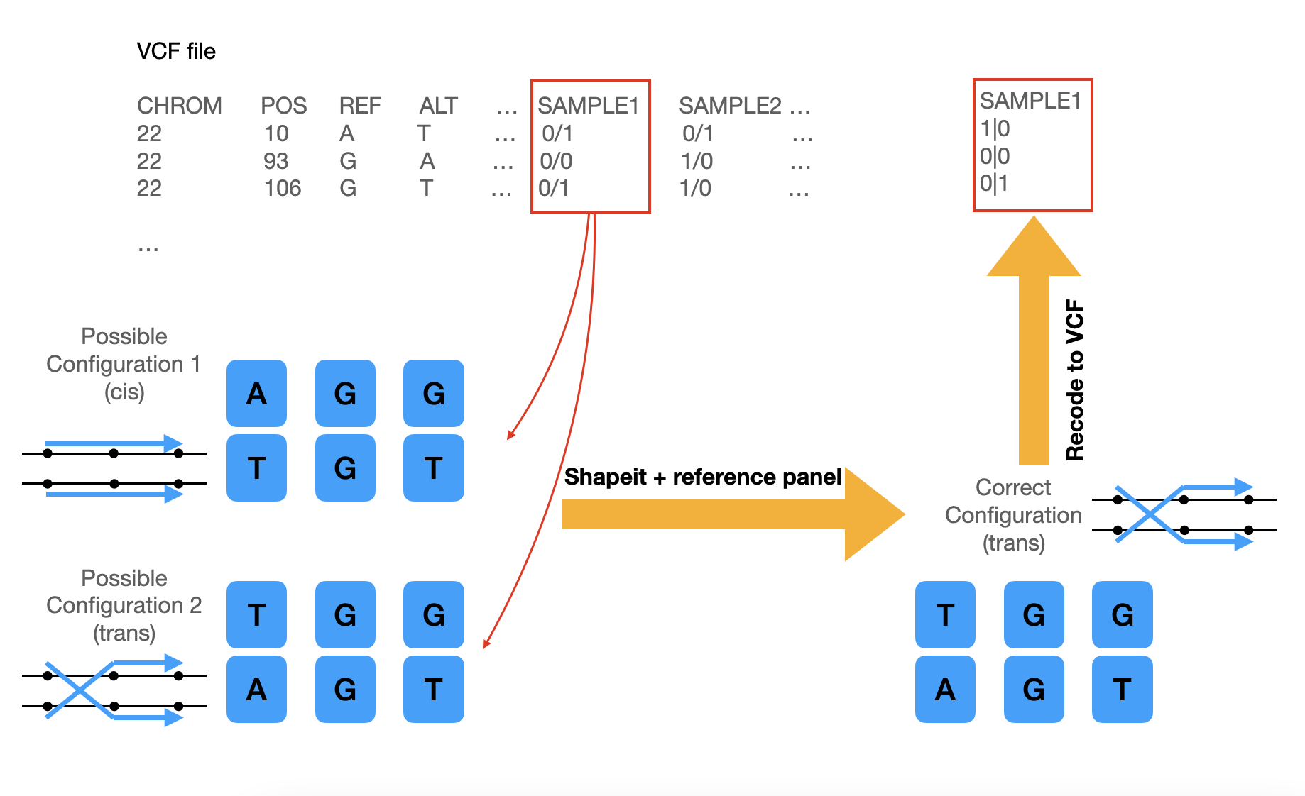
Cohort genotype data is commonly provided in VCF format. However, despite the human genome being diploid, sequencing/genotyping technology can only reveal genotype presence, not their orientation (haplotype). This means we lack information on which allele resides on which chromosome strand. Statistical phasing aims to reconstruct allele configurations along a chromosome, as depicted in the diagram.

Notice that each entry is separated with slash (e.g. 0/1), and that means the VCF file is unphased. By performing phasing, we will figure out the most likely configuration of allele positions. After performing the following steps, we should get a phased VCF file, with the slash substituted by a vertical bar (e.g. 1|0) which indicates that the data is phased.

Several tools has been developed for statistical phasing, here we use SHAPEIT5 to perform phasing using a reference haplotype panel.

As previously mentioned, the following steps and flags are only indicated here for demonstration purposes, and does not serve to provide a comprehensive use of SHAPEIT5. For example, phasing can be performed without SHAPEIT5 as well.

Please refer to the SHAPEIT5 manual here to better understanding the functionalities about SHAPEIT5.

A. Adding INFO/AC and INFO/AN tags required by SHAPEIT5 pre-phasing

# Add AC/AN tags in input file
bcftools +fill-tags admixed_cohort/ASW.unphased.vcf.gz \
-Oz \
-o admixed_cohort/ASW.unphased_mod1.vcf.gz \
-- -t AN,AC

# Index file
bcftools index admixed_cohort/ASW.unphased_mod1.vcf.gz

B. Perform SHAPEIT5 phasing

This step aims to phase the common variants in the input file using the reference panel. The required static bins (phase_common_static) for SHAPEIT5 can be downloaded here.

The --thread argument is optional and should be adjusted based on the number of cores available on your system. This is a computationally expensive step, especially in cases of real datasets, and thus multi-threading is recommended.

phase_common_static \
--input admixed_cohort/ASW.unphased_mod1.vcf.gz \
--reference references/TGP_HGDP_QC_hg19_chr22.vcf.gz \
--region 22 \
--map references/chr22.b37.gmap.gz \
--output admixed_cohort/ASW.phased.bcf \
--thread 8

# Convert output BCF to VCF and index it
bcftools convert \
-Oz \
-o admixed_cohort/ASW.phased.vcf.gz \
admixed_cohort/ASW.phased.bcf

bcftools index \
admixed_cohort/ASW.phased.vcf.gz

# Delete redundant file
rm admixed_cohort/ASW.phased.bcf admixed_cohort/ASW.phased.bcf.csi

The program will display critical information regarding input and output files, including the number of variants present, variants removed due to lack of overlap between the main input and reference panel, and the number of identified samples.

Reading genotype data:
  * VCF/BCF scanning done (13.13s)
      + Variants [#sites=182525 / region=22]
         - 34621 sites removed in main panel [not in reference panel]
         - 11249 sites removed in reference panel [not in main panel]
      + Samples [#target=61 / #reference=1572]

Note: If using a reference panel, ensure that your panel is phased. If you intend to use an unphased reference panel, consider first running SHAPEIT5 phasing on the reference panel or joint-phasing your cohort and reference populations in a combined file.

SHAPEIT5 users have the option to phase the dataset without a reference panel. The necessity of a reference panel depends on your input cohort and the potential value it may add. Additional information can be found on the SHAPEIT5 website.

Local Ancestry Inference

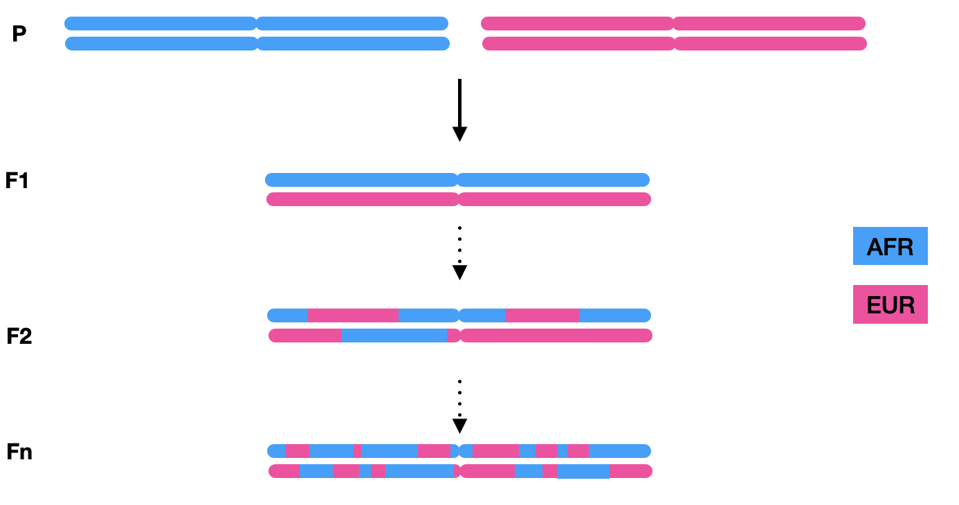
To conduct local ancestry inference, a homogeneous phased reference panel representing relevant ancestries and a phased admixed cohort VCF file are required. Admixed populations exhibit chromosomes composed of mosaic ancestral tracts, as different chromosomal segments are inherited from multiple ancestries. The length of these tracts is influenced by the demographic history of the population, with shorter tracts resulting from more recent admixture events, as recombination breaks down tracts over generations.

For instance, in a two-way admixed AFR-EUR population, illustrated below, the first generation inherits one full chromosome copy from each ancestry. Subsequent generations undergo recombination during meiosis, resulting in chromosomes fragmented into smaller ancestral segments.

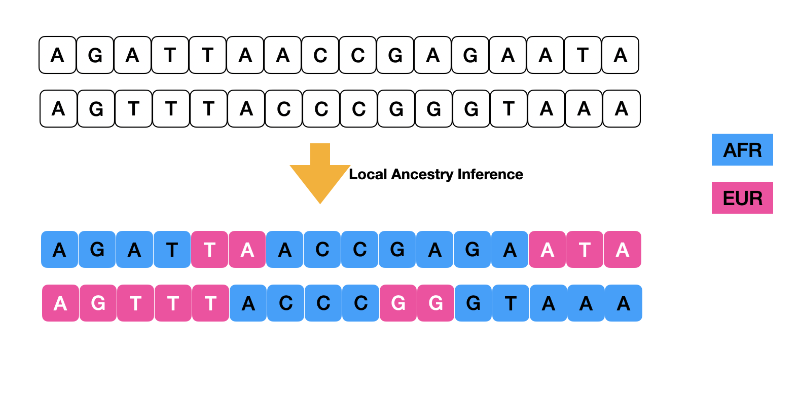
The objective of local ancestry inference is to assign ancestry origins to each genomic segment within individuals’ chromosomes. In the subsequent analysis of the Tractor pipeline, local ancestry information facilitates a deeper understanding of genotype-phenotype associations.

For local ancestry inference, we utilize RFMix2, known for its accuracy in two-way AFR/EUR admixed populations. RFMix2 requires the following parameters and generates four files (ASW.deconvoluted.fb.tsv, ASW.deconvoluted.msp.tsv, ASW.deconvoluted.rfmix.Q, ASW.deconvoluted.sis.tsv), most of which are utilized in downstream analysis. It is advisable to validate the performance of local ancestry inference by reviewing the global ancestry fractions provided in ASW.deconvoluted.rfmix.Q to ensure alignment with expected global ancestry proportions in your target cohort.

rfmix \
-f admixed_cohort/ASW.phased.vcf.gz \
-r references/TGP_HGDP_QC_hg19_chr22.vcf.gz \
-m references/YRI_GBR_samplemap.txt \
-g references/chr22.genetic_map.modified.txt \
-o admixed_cohort/ASW.deconvoluted \
--chromosome=22

Now that you have your local ancestry calls, you’re all set for Tractor! In the next post, we’ll illustrate how you can optionally enhance phasing by correcting switch errors that typically occur in phasing. Alternatively, if your objective primarily involves understanding variant-level tests (e.g., Tractor GWAS), you can proceed directly to Step 2: Extract tracts.