Tractor-tutorial
![]()
Compared to the standard GWAS model, Tractor takes local ancestry into account and therefore may help improve discovery power when there are (LD, MAF, or effect size) differences across ancestries, as well as better localizing top hits, and providing more accurate effect size estimates. In the previous step, we demonstrated how to perform local ancestry inference using Rfmix. Now, we will process the RFmix output files to generate more interpretable intermediate files which will be used in statistical modeling.
Prerequisites
Download Tractor Scripts
Tractor scripts are readily available on the Tractor GitHub repository and can be easily cloned. All scripts utilized in this tutorial are accessible in the scripts/ directory.
git clone https://github.com/Atkinson-Lab/Tractor.git
Here, we showcase the fundamental functionality of these scripts. However, we recommend referring to the README for Tractor to explore additional functionalities beyond those outlined here.
Verify files in admixed_cohort directory
The previous Phasing step should have generated the following files.
ASW.unphased.vcf.gz[.csi]
ASW.unphased_mod1.vcf.gz[.csi] # Modified to include AC/AN tags
ASW.phased.vcf.gz[.csi]        # SHAPEIT5 phased data
The ASW.phased.vcf.gz file, converted from standard SHAPEIT5 output will serve as an argument for extract_tracts.py.
Additionally, after performing local ancestry inference with RFMix2, the following files should have been generated:
ASW.deconvoluted.fb.tsv
ASW.deconvoluted.msp.tsv
ASW.deconvoluted.rfmix.Q
ASW.deconvoluted.sis.tsv
The ASW.deconvoluted.msp.tsv file, containing the most probable ancestral assignments for all variants in each individual within the cohort, will be utilized as an argument for extract_tracts.py.
Extract Tracts
We offer a script capable of extracting risk allele information and local ancestry simultaneously.
python3 extract_tracts.py \
--vcf admixed_cohort/ASW.phased.vcf.gz \
--msp admixed_cohort/ASW.deconvoluted.msp.tsv \
--num-ancs 2
4 files will be generated:
ASW.phased.anc0.dosage.txt
ASW.phased.anc0.hapcount.txt
ASW.phased.anc1.dosage.txt
ASW.phased.anc1.hapcount.txt
What happened under the hood?
Let’s take a peek at our input files ASW.phased.vcf.gz and ASW.deconvoluted.msp.tsv.
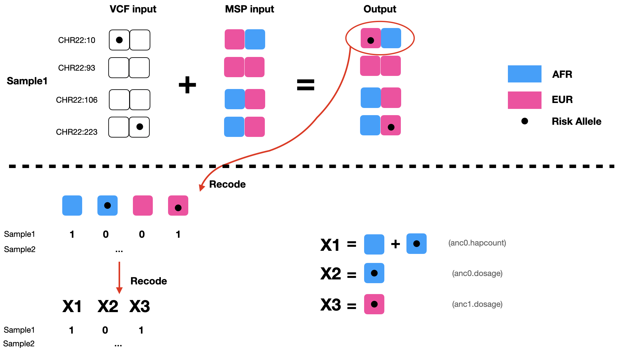
The phased vcf file contains haplotype information for each individual in the cohort. Reference alleles are represented with a 0, alternate alleles (often assumed to be the risk allele) as a 1. Here you can see the first 4 variants in chromosome 22 for SAMPLE1:
CHROM POS REF ALT SAMPLE1   ...
22    10  A   T   1|0       ...
22    93  G   A   0|0       ...
22    106 G   A   0|0       ...
22    223 G   A   0|1       ...
...
The msp file contains local ancestry information for each person, for each of their two chromosome strands. Notice its coordinates are in a different format from the vcf file – the msp file uses a window to specify LA information. For example, the first row of the following msp file is telling us this: for SAMPLE1, strand0 from position 1 to position 52 is inherited from EUR ancestry (ancestry 1 in our input files) and strand 1 from position1-position52 is inherited from an AFR background (anc0 in our input files). Generally, RFmix orders ancestries alphabetically, so the first will be anc0, the second anc1, etc.
AFR=0       EUR=1
CHROM SPOS  EPOS SAMPLE1.0 SAMPLE1.1   ...
22    1     52  1         0       ...
22    52    101 1         1       ...
22    101   190 0         1       ...
22    190   283 0         1       ...
...
By checking both files simultaneously, we can figure out the local ancestry (LA) background of each of the alleles in our dataset, as the upper portion of the following diagram shows. To represent both LA and risk allele information, we need to recode each variant into 4 columns, with each column represents a unique combination of LA and risk allele (AFR-nonRisk, AFR-Risk, EUR-nonRisk, EUR-Risk). In the diagram below, at the first variant, SAMPLE1 has one copy of AFR-nonRisk, and one copy of EUR-Risk, and therefore will be encoded to [1,0,0,1].
To further compress the information, extract_tracts.py did an additional step – talling the total number of copies of AFR local ancestry for each variant for each person. This can be thought of as adding AFR-nonRisk and AFR-Risk.

Running ExtractTracts.py on our toy dataset will generate 4 files, and 3 of them will be used in the next step for statistical modeling in the Tractor GWAS. You can read about the other files on the Tractor Wiki for this script here.
ASW.phased.anc0.hapcount.txt        (used as X1)
ASW.phased.anc0.dosage.txt          (used as X2)
ASW.phased.anc1.dosage.txt          (used as X3)
Now we are ready to run Tractor GWAS! We have recently developed scripts for Tractor that may be used either on a local computer or in a high-perfomance computing setting (Local Tractor). These are subtlely refined over the originally released cloud native scripts (we fixed a few edge cases/bad behaviors). Should Tractor need to be run on an extremely large dataset, however, we also have developed scabable cloud-native scripts written in Hail. The user may select which of the two versions of Tractor GWAS they wish to run with the links below. For this tutorial, we recommend using Local Tractor.